Simulate labels with difficulty

This is an example of simulation using the peerannot library that considers tasks’ difficulty. The discrete-difficulty strategy simulates the following setting (here presented with $K=3$ classes for simplicity):

Discrete-difficulty simulation

Each task is assigned a true label $y_i^\star$ and a difficulty level $d_i$ in $\{$ easy, hard, random $\}$. Each worker is either good of bad

• If the task is easy, every worker answers correctly: $y_i^{(j)}=y_i^\star$
• If the task is random, every worker answers randomly: $\mathbb{P}(y_i^{(j)}=m\vert y_i^\star=k) = \frac{1}{K}$.
• If the task is hard, each worker $w_j$ is assigned a confusion matrix $\pi^{(j)}$ where $\pi^{(j)}_{k,m} = \mathbb{P}(y_i^{(j)}=m\vert y_i^\star=k)$:
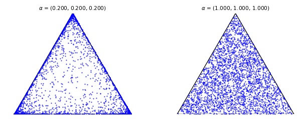
  • if the worker is good, each row of the confusion matrix is simulated using a $\mathcal{D}\text{irichlet}(\alpha=[0.2, 0.2, 0.2])$ with maximum located at $y_i^\star$
  • if the worker is bad each row of the confusion matrix is simulated using a $\mathcal{D}\text{irichlet}(\alpha=[1, 1, 1])$, i.e. the uniform distribution over the simplex. The final answer is then drawn from the Multinomial $\big(\pi^{(j)}_{y_i^\star, \bullet}\big)$

If you have a worker of profile fixed that does not rely on Dirichlet distributions, peerannot works too! Simply store your confusion matrices in an .npy file containing an np.ndarray of shape (n_worker, K, K) and then use the --matrix-file_path_to_matrix_file.npy argument to use your own confusion matrices.

Run the simulation

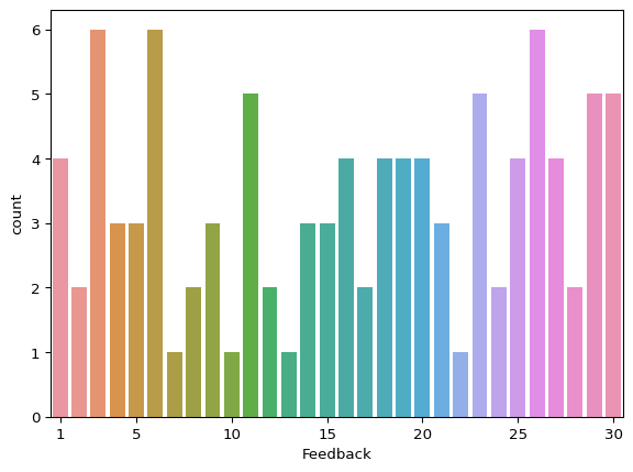
Let us run a simulation with $n_{\texttt{worker}}=30$ workers, $n_{\texttt{task}}=100$ tasks with $K=3$ classes. Each task receives a random number of votes between $1$ and $n_{\texttt{worker}}$ using the key imbalance-votes

The maximum number of tasks per worker / label per task can be modified using workerload/feedback parameters.

Results are stored in the folder ./temp/test_discrete_difficulty. There are $0.7\cdot n_{\texttt{worker}}$ good workers. The probability for a task to be random is set to $p_{\text{random}}=0.3$, and the ratio of good over hard tasks is set to $r=0.4$ i.e. the choice between easy, hard and random difficulty $d_i$ follows:

We set the seed to $3$ for reproducibility.

!peerannot simulate --n-worker 30 --n-task 100  -K 3 \
                    -s discrete-difficulty \
                    --folder ./temp/test_discrete_difficulty/ \
                    -r 0.7 --ratio-diff 0.4 --random 0.3 \
                    --imbalance-votes \
                    --seed 5;

Explore results

Workers’ answers

The simulation created the dictionary of answers for each task and worker in answers.json:

import numpy as np
import json
import seaborn as sns
from pathlib import Path

dir_ = Path.cwd() / "temp" / "test_discrete_difficulty"

with open(dir_ / "answers.json", "r") as all_ans:
    answers = json.load(all_ans)  # warning: keys are string
true_labels = np.load(dir_ / "ground_truth.npy")

sns.countplot(data={
  "votes_repartition": [len(t) for t in answers.values()]
  }, x="votes_repartition")
plt.xticks([0] + list(range(4, 30, 5)), [1] + list(range(5, 31, 5)))
plt.xlabel("Feedback")
plt.show()

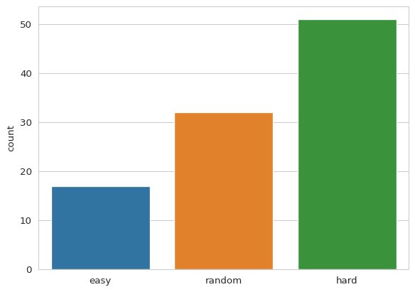
Task difficulty

The difficulty of each task is accessible in difficulties.npy:

sns.set_style("whitegrid")
diff = np.load(dir_ / "difficulties.npy")
sns.countplot(data={"difficulty": diff}, x="difficulty")
plt.show()

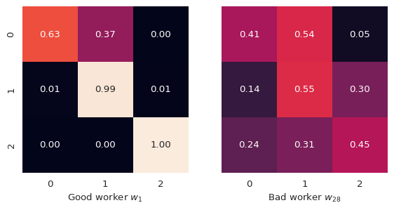
Confusion matrices

Finally, confusion matrices $\pi^{(j)}$ are stored in matrices.npy.

The confusion matrix of a good worker is always diagonally dominant.

pi = np.load(dir_ / "matrices.npy")
fig, axs = plt.subplots(1, 2, sharey=True)
sns.heatmap(pi[1], ax=axs[0], annot=True, fmt=".2f", square=True, vmin=0, vmax=1, cbar=False)
sns.heatmap(pi[28], ax=axs[1], annot=True, fmt=".2f", square=True, vmin=0, vmax=1, cbar=False)
axs[0].set_xlabel("Good worker $w_1$")
axs[1].set_xlabel("Bad worker $w_{28}$")
plt.show()